PID Control
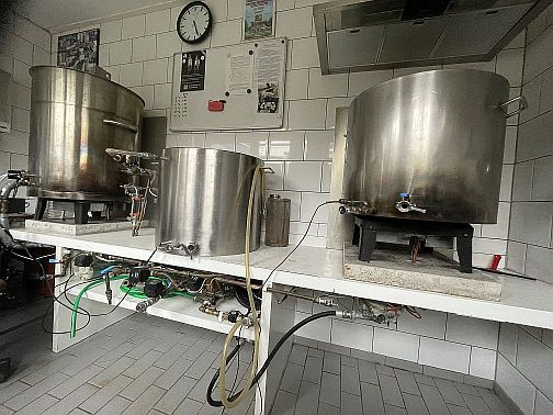
Why would a home-brewer need a separate page just on control engineering? If you have a RIMS / HERMS brewing setup and you buy a neat little box that does all the tricks, why bother with PID control? As a home-brewer you have to understand a little how PID control works, because you can easily end up with a non-optimum PID controller, which causes significant temperature overshoots or very slow responses.
Suppose you think that you can do without PID control, you just switch off the heater when the temperature has reached its value. What happens in this situation is that the temperature in your setup continues to rise significantly. So you end up with a large overshoot. The heater should be switched off gradually, long before the final temperature is reached. That is where a controller comes in and the PID controller is the most common used one. PID stands for Proportional, Integral and Derivative. If you look at the insides of a PID controller, you see that it indeed consists of three paths. It used to be very common to build such a PID controller with discrete electronics, but nowadays every PID controller is realised in software, making it a digital PID controller. Such a digital PID controller is contained in the ready-for-use devices that you can buy. And if you have read this page, you understand that it is a high price to pay for only a few lines of code (so building your own PID controller can be rewarding).
In the remainder of this page I will try to explain the following items:
- 1. PID Control Basics: some basic theory on PID control
- 2. Implementation of a PID controller: a real PID controller with C source code
- 3. Tuning the PID controller: finding the optimum parameters for your brewing system. This paragraph consists of the following sub-paragraphs:
If you have an interest in building your own PID controller, check out my hardware and software pages. These pages shows the complete design and build of a brewing system with a PID controller.
1. PID Control Basics
The key parts of a PID control loop are shown in the figure below.
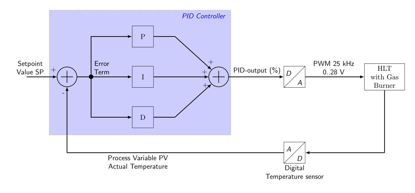
- Setpoint value: The desired or required value for the process variable. In the brewing setup, the setpoint value is derived from the mash scheme. If a particular mash rest has finished, the setpoint-value is set to the next, higher, temperature reference.
- Process variable: a measured value of some physical property. In the brewing setup, this is the measured temperature from the HLT.
- Error Term: the algebraic difference between the process variable and the setpoint value. This is the control loop error, and is equal to zero when the process variable is equal to the setpoint (desired) value. A well-behaved control loop is able to maintain a small error term magnitude.
- PID-output: The output of the PID controller, which is typically a value between 0 % and 100 %. This signal controls the amount of power to dissipate in the HLT.
- D/A: The Digital to Analogue Converter (DAC). It transforms the digital value into an analogue signal. In the brewing system, this is done with a PWM signal made by a timer in the microcontroller. It has a frequency of around 25 kHz, the 0..5 Volt PWM signal from the microcontroller is amplified to 0..28 Volt, which is the proper voltage-level for the gasburner valve.
- A/D: The Analogue to Digital Converter (ADC). It transforms the analogue value into its digital representation. The brewing system uses a digital temperature sensor, the LM92. This neat little device has a built-in A/D converter, so an external one is not necessary.
The Proportional-Integral-Derivative (PID) algorithm is widely used in process control. The PID method of control adapts well to electronic solutions, whether implemented in analogue or digital (CPU) components. The brewing program implements the PID equations digitally by solving the basic equations in software. Basically, there are two types of PID controls:
- PID Position Algorithm : The control output is calculated so it responds to the displacement (position) of the process variable from the setpoint value (error term). The control output is an absolute value. Example: the control output is set to 5 %, the heater is then switched on for 5 % of its time.
- PID Velocity Algorithm: The control output is calculated to represent the rate of change (velocity) for the process variable to become equal to the setpoint value. The control output is a relative value (relative to the previous value of the control output). Example: the control output is set to 5 % and the previous value of the control output was 55 %. The new control output will be equal to 55 % - 5 % = 50 %. The heater is then switched on for 50 % of its time (and not 5 %).
Within the brewing program, the PID Velocity Algorithm is chosen (which is also the algorithm that is used in most digital PID controllers). Another important feature of a control loop is whether it is a direct-acting loop or a reverse-acting loop:
- Direct-Acting Loop: the process has a positive gain, meaning that when the control output is increased, the power is increased as well, which results in an increase of temperature. This is the case in our brewing setup.
- Reverse-Acting Loop: the process has a negative gain, meaning that when the control output is increased, the process variable would decrease. This is commonly found in refrigeration controls, where an increase in the cooling input causes a decrease in the process variable (temperature). Accordingly, reverse-acting loops are sometimes called cooling loops.
In the figure shown above, three parallel paths were shown in the PID-loop calculation block:
- Proportional: The proportional term simply responds proportionally to the current size of the error. This loop controller calculates a proportional term value for each PID calculation. When the error is zero, the proportional term is also zero.
- Integral: The integrator (or reset) term integrates (sums) the error values. Starting from the first PID calculation (after the controller was released), the integrator keeps a running total of the error values.
- Derivative: The derivative (or rate) term responds to change in the current error value from the error used in the previous PID calculation. Its job is to anticipate the probable growth of the error and generate a contribution to the output in advance.
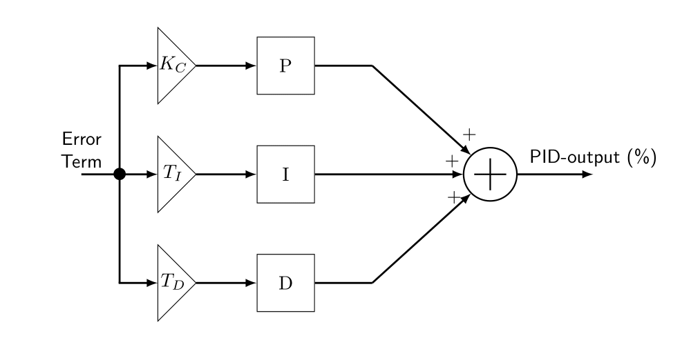
The P, I and D terms work together as a team. To be able to control these terms, each term has a programmable gain:
- Kc: The proportional gain. Some textbooks also call this Kp. The unity (in our brewing setup) is % / °C.
- Ti: The time-constant for the integral gain. Some textbooks also define this as: Ti = Kc / Ki. The unity (in our brewing setup) is seconds.
- Td: The time-constant for the derivative gain. Some textbooks also define this as: Td = Kc / Kd. The unity (in our brewing setup) is seconds.
- In fact, there is another parameter that is also important and that is the sample time Ts. The sample time Ts is defined as the time between two calls to the PID-controller. In our brewing system, the sample-time Ts for the PID controller is set to 5 seconds (meaning that once every 5 seconds, a call to the PID controller is made).
There is one more remark to make about the type of PID controller (for details and more background, please read the PID controller Calculus document with full C source):
- Type A PID Controller: This is the type of PID controller in the picture above, also called Textbook PID. Not many engineers prefer this type. This is because the D term is also dependent of the error term. And since the error term is equal to the setpoint value minus the process variable (the actual HLT temperature), it means that it also reacts to a change in setpoint value. This is not desired, since we want to change the setpoint value without disturbing the controller output.
- Type B PID Controller: In a type B PID controller, the setpoint value is removed from the D term. This will lead to a scheme where the D term is fed only with the process variable (the actual HLT temperature) and no longer with the error term.
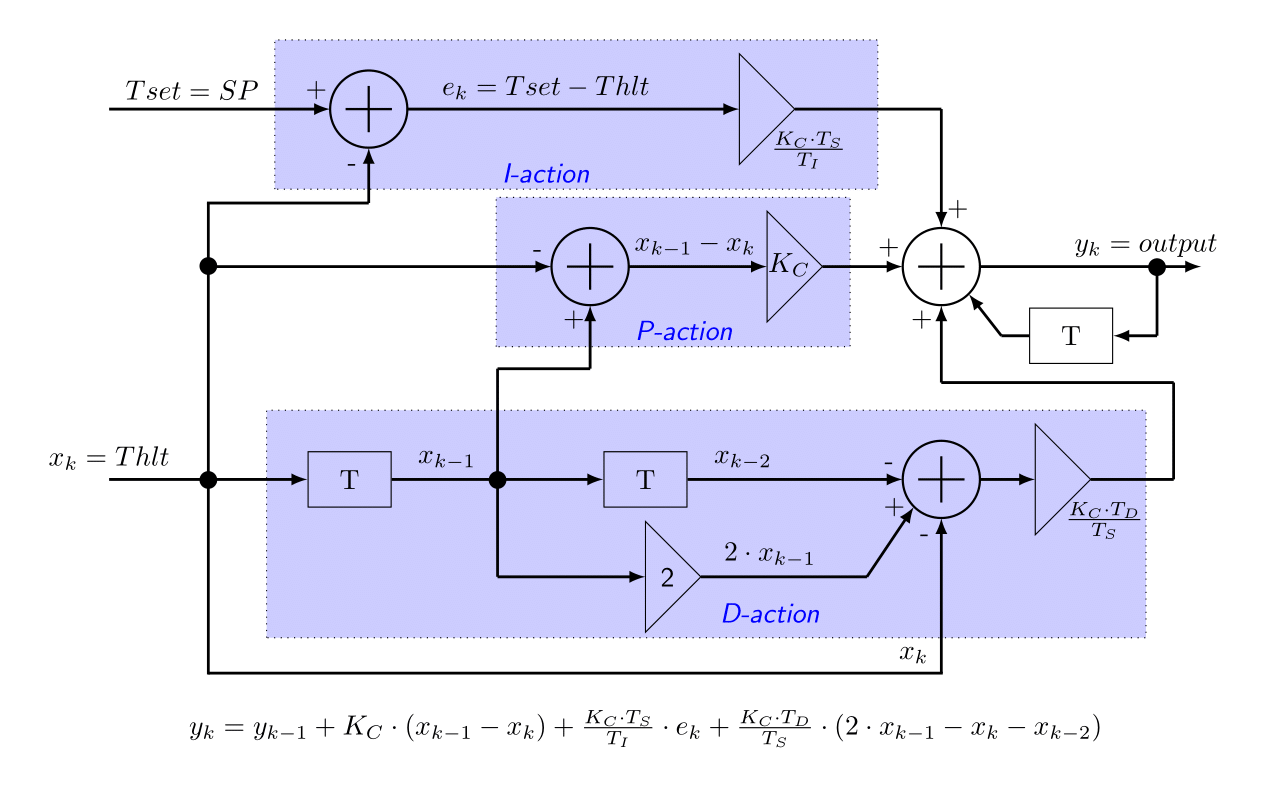
- Type C PID Controller: The type B PID controller can be further improved by also removing the error term from the P term. In a type C controller, the error term is still fed to the I-term, but the P- and D-term are only dependent of the process variable (the actual HLT temperature).
Some industrial PID controllers allow users to select any of these types. However, if a type C PID controller is available, you should select this one. A system blockdiagram of such a type-C controller is given in the figure below. The separate P, I and D-actions are clearly seen. This is also the controller that is used in the brewing system.
 Back to the Top of the Page
2. Implementation of a PID controller
Many different implementations are possible. In fact, every modern PLC may have a different implementation of a PID controller, which makes things confusing. Deriving a form suitable for implementation requires a lot of Calculus. I did all this, so if you are really looking for a derivation of the PID controller implementation given here, together with the full C source code (so you can directly build your own controller), please read this document: PID Controller Calculus with full C source code. However, if you are not really into math and you are only interested in an actual implementation, so that you can use this in your own software, then read this paragraph. The document also contains the full C source for the PID controllers. Here, we will be using a PID velocity algorithm of Type C, which is direct-acting and has no filtering of the D-action. This is the so-called Takahashi PID controller and is probably the best way to implement a PID controller. The figure below shows the actual C code. This figure makes it easy (I hope) to transform the code to your own favourite programming language (the gray lines of text are comments). Based on this example, it is relatively easy to make this into a 'real' Takahashi type C PID controller.
/*==================================================================
  Function name: pidInit(), pidCtrl()
  Author       : Emile
  ------------------------------------------------------------------
  Purpose : This file contains the main body of the PID controller.
            For design details, please read the Word document
            "PID Controller Calculus".

            In the GUI, the following parameters can be changed:
            Kc: The controller gain
            Ti: Time-constant for the Integral Gain
            Td: Time-constant for the Derivative Gain
            Ts: The sample period [seconds]
  ==================================================================*/
#include "pid_reg_web.h"
#include

void pidInit(pidPars *p, double Kc, double Ti, double Td, double Ts)
/*------------------------------------------------------------------
  Purpose  : This function initialises the PID controller.
  Variables: p : pointer to struct containing PID parameters
             Kc: the controller gain [%/C]
             Ti: integral time-constant [sec.]
             Td: differential time-constant [sec.]
             Ts: sample-time period [sec.]

                   Kc.Ts
             ki =  -----   (for I-term)
                    Ti

                       Td
             kd = Kc . --  (for D-term)
                       Ts

  Returns  : No values are returned
  ------------------------------------------------------------------*/
{
    p->kp = Kc;
    if (Ti < 1e-3)
         p->ki = 0.0;
    else p->ki = Kc * Ts / Ti;
    if (Ts < 1e-3)
         p->kd = 0.0;
    else p->kd = Kc * Td / Ts;
    p->xk_2 = p->xk_1 = p->yk = 0.0;
} // pidInit()

double pidCtrl(double xk, double tset, pidPars *p, int vrg)
/*------------------------------------------------------------------
  Purpose  : This function implements the Takahashi Type C PID
             controller: the P and D term are no longer dependent
             on the set-point, only on PV (which is Thlt).
             This function should be called once every TS seconds.
  Variables:
        xk : The input variable x[k] (= measured temperature)
      tset : The setpoint value for the temperature
        *p : Pointer to struct containing PID parameters
        vrg: Release signal: 1 = Start control, 0 = disable PID controller
  Returns  : yk : PID controller output y[k] in % [0..100]
  ------------------------------------------------------------------*/
{
   if (vrg)
   {
      //--------------------------------------------------------------------------------
      // Takahashi Type C PID controller (NO filtering of D-action):
      //
      //                                    Kc.Ts        Kc.Td
      // y[k] = y[k-1] + Kc.(x[k-1]-x[k]) + -----.e[k] + -----.(2.x[k-1]-x[k]-x[k-2])
      //                                      Ti           Ts
      //
      //--------------------------------------------------------------------------------
      p->pp  = p->kp * (p->xk_1 - xk);                 // Kc.(x[k-1]-x[k])
      p->pi  = p->ki * (tset - xk);                    // (Kc.Ts/Ti).e[k]
      p->pd  = p->kd * (2.0 * p->xk_1 - xk - p->xk_2); // (Kc.Td/Ts).(2.x[k-1]-x[k]-x[k-2])
      p->yk += p->pp + p->pi + p->pd;                  // add y[k-1] + P, I & D actions to y[k]
   }
   else { p->yk = p->pp = p->pi = p->pd = 0.0; }

   p->xk_2  = p->xk_1;  // x[k-2] = x[k-1]
   p->xk_1  = xk;       // x[k-1] = x[k]

   // limit y[k] to a maximum and a minimum
   if (p->yk > PID_OUT_HLIM)
   {
      p->yk = PID_OUT_HLIM;
   }
   else if (p->yk < PID_OUT_LLIM)
   {
      p->yk = PID_OUT_LLIM;
   } // else
   return p->yk;
} // pidCtrl()
There are a few remarks to make about this implementation:
- This function is called once every TS seconds, with Ts being set to 20 seconds in my brewing program. It means that a new value for the PID controller output is calculated every 20 seconds.
- The actual temperatures are read in every second. These temperatures are filtered and then passed to this function (as xk).
- The values of Kc, Ti, Td and Ts can be adjusted by the brewer (see the GUI section on the software page).
- The extension _1 to several variables (e.g. xk_1) indicates the previous version of that variable. For example: xk_1 means the value of xk during the previous call to this function (20 seconds ago). Same with the extension _2 (which was the value 2 * 20 seconds ago).
- Prior to calling pidCtrl() for the first time, it has to be initialised. For this reason, the function pidInit() was created which calculates the value of certain constants. This routine has to be called whenever one or more parameters have been changed.
- The code below is written in the C programming language. There's also a C++ version of it and that one is actually used in the brewing program. Check the Github repository if you are interested in those sources, the PID controller class can be found in the files controlobjects.cpp and controlobjects.h
Please let me know if you find this listing easy or difficult to read. I would be interested to hear about it.
A header file (.h) is normally created for every C file. Such a file contains the function prototypes and important definitions / constants. If you want to use these function, you would typically include this header file into your C project.
#ifndef PID_REG_H
#define PID_REG_H
/*==================================================================
  File name    : pid_reg_web.h
  Author       : Emile
  ------------------------------------------------------------------
  Purpose : This is the header file for pid_reg_web.c
  ==================================================================*/

#define PID_OUT_HLIM (100.0) /* PID Controller Upper limit (%) */
#define PID_OUT_LLIM   (0.0) /* PID Controller Lower limit (%) */

//------------------------------------------------------------
// By using a struct for every PID controller, you can have
// more than 1 PID controller in your program.
//------------------------------------------------------------
typedef struct _pidPars
{
   double kp;   // Internal Kp value
   double ki;   // Internal Ki value
   double kd;   // Internal Kd value
   double pp;   // debug value for monitoring of P-action
   double pi;   // debug value for monitoring of I-action
   double pd;   // debug value for monitoring of D-action
   double yk;   // y[k]  , value of controller output (%)
   double xk_1; // x[k-1], previous value of the input variable x[k] (= measured temperature)
   double xk_2; // x[k-2], previous value of x[k-1] (= measured temperature)
} pidPars; // struct pidParams

//----------------------
// Function Prototypes
//----------------------
void   pidInit(pidPars *p, double Kc, double Ti, double Td, double Ts);
double pidCtrl(double xk, double tset, pidPars *p, int vrg);
#endif
As an example of how to call these routines from within a C-program, the code below is given. The function pidInit() is called first with the actual PID parameters and then the controller itself is called (the function pidCtrl()). The pidCtrl() function needs an actual temperature, a setpoint value, the struct with all controller parameters and a release signal. The controller will start controlling only, when this release signal is set to 1.
#include
#include
#include "pid_reg_web.h"

int main()
{
    pidPars p;          // Create a struct for pidPars
    double out  = 0.0;  // PID controller output
    double temp = 30.0; // Actual temperature
    double sp   = 32.0; // Setpoint temperature

    // Call pidInit with the proper control parameters
    pidInit(&p, 80.0, 280.0, 45.0, 20.0); // p, Kc, Ti, Td, Ts

    // Call the actual controller every Ts seconds
    out = pidCtrl(temp, sp, &p, 0); // x[k], SP, p, vrg
    out = pidCtrl(temp, sp, &p, 0); // call this function every Ts seconds
    // The PID-controller is enabled by setting vrg to 1
    out = pidCtrl(temp, sp, &p, 1); // Controller is released
    out = pidCtrl(temp, sp, &p, 1); //
    return 0;
} // main()
3. Tuning the PID controller
Tuning the PID controller means finding values for Kc, Ti and Td, such that the PID controller responds quickly to changes in setpoint value and/or temperature, while minimising any overshoot in temperature. Tuning a PID controller is always necessary, even if you bought a ready-to-use PID controller. The advantage of such a ready-to-use PID controller is that they contain an auto-setup function, which finds the optimum values automatically for you (well, most of the time). But even such a ready-to-use PID controller uses the same algorithms as the ones I describe here. So this information might also be useful to you if you did not create your own PID controller, but bought one. In order to understand the specific measurements which we are about to do, some terms and definitions have to be explained:
- Open loop response: the open loop response means that the PID controller output is set to a fixed value (e.g. 20%) and the response of the system (in our case the HLT temperature) is measured. The term open loop comes from the fact that the PID controller is not in control, but set to a fixed value, the loop is not closed.
- Closed loop response: the closed loop response means that the PID controller is enabled and that we apply a step to the setpoint value (the HLT temperature reference). Then we measure how the PID controller is doing by measuring the response of the system (the HLT temperature). For example: we could set the HLT reference temperature from 20 °C up to 50 °C, thereby creating a step of 30 °C.
- Dead-Time (TD): the dead-time of the system is the time delay between the initial response and a 10 % increase in the process variable (which is the HLT temperature in our case). Unity is given in seconds.
- Normalized slope (a): the normalized slope of the step response is the increase in temperature per second per percentage of the PID controller output. Stated in a formula: a = change in temperature divided by time-interval divided by PID controller output.
- Gain (K): the gain of the HLT system. We can model our HLT system as having one input (the PID controller output in %) and one output (the HLT temperature). The Gain of this HLT system is then defined as output divided by input and has a unity of °C / %.
- Time-constant (tau): the time-constant of the system is another important parameter of the system. It describes how quick the temperature will increase, given a particular output of the PID controller. Unity is given in seconds.
3.1 Determine Dead-Time and normalized slope of the HLT system
Manually set the PID-controller output to a certain value (e.g. 20 %). In case of a heavy load, 100 % is recommended (more accurate), but if you do not know the performance of the system, a lower value to start with is better. The temperature starts to increase and follows the following curve:
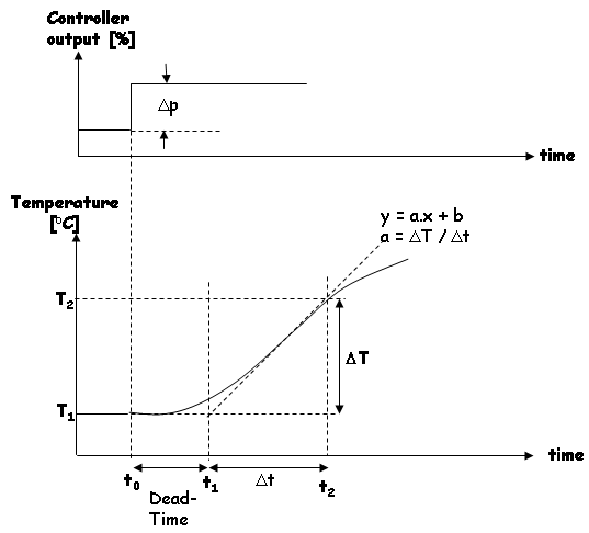
After doing this experiment with my HLT system (90 L of water, no lid on the pan, controller output set to 100 %, heating element only), combined with some regression analysis (for more accuracy), I found out that the dead-time for my HLT system is equal to 115 seconds. During the experiment, the temperature change was 0.4 °C per minute when the PID controller output was set to 100 %. The normalized slope a is therefore equal to 0.004 °C / (%.minute) or 6.68E-5 °C/(%.s). BUT... since I switched over to gas-burners, and more recently, to a new HLT kettle, I may have to do this experiment again!.
3.2 Determine Time-Constant of the HLT system
Because of the large time-constant presumably present in the HLT system, the previous experiment is not very accurate in determining the dead-time as well. This is the mean reason to conduct two experiments (theoretically, the step-response would give you all the required information to determine the three parameters). Manually set the PID-controller output to a certain value (e.g. 20 %). The temperature starts to increase and follows the following curve:
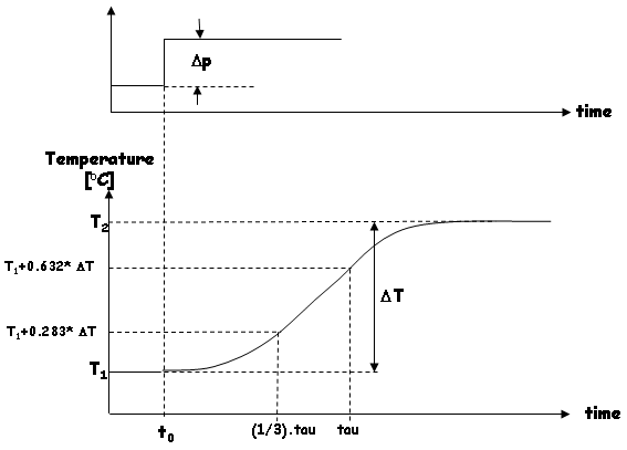
The difference with the previous experiment is that we let the PID controller settle, meaning that the HLT temperature will converge to a new value (in my experiment, this took a complete day, because I wanted it as reliable as possible). After doing this experiment with my HLT system (90 L of water, no lid on the pan, controller output set to 20 %, heating element only), I collected the following data:
- t0 = 09:49:04, T1 = 19.20 °C
- T2 = 52.99 °C, T2 - T1 = 33.79 °C
- T1 + 0.283 * (T2 - T1) = 28.76 °C. Check the HLT temperature graph when this temperature was reached. In the experiment, this temperature was reached 6599 seconds after the start (t0). Therefore: tau/3 = 6599 seconds.
- T1 + 0.632 * (T2 - T1) = 40.56 °C. Check the HLT temperature graph when this temperature was reached. In the experiment, this temperature was reached 16573 seconds after the start (t0). Therefore: tau = 16573 seconds.
- Solving tau from the previous two results: tau - tau/3 = 16573 - 6599 <=> (2/3) * tau = 9974 <=> tau = 14961 seconds.
- The Gain is calculated directly from this data as well: Gain = (T2 - T1) / 20 % = 33.79 °C; / % = 1.69 °C / %.
3.3 Calculate the Optimum values for the PID controller (Kc, Ti and Td)
A summary of the results from the two experiments for my particular HLT system:
- Dead-Time TD = 115 seconds
- Normalized slope a = 6.68E-5 °C/(%.s).
- Gain (K) = 1.69 °C / %.
- Time-constant (tau) = tau = 14961 seconds.
There are a few well-known algorithms that calculate the optimum settings for a PI and a PID controller. These algorithms calculate a value for Kc, Ti and Td based upon the values found for TD, a, K and tau. The algorithms are:
- Ziegler-Nichols Open Loop
- Ziegler-Nichols Closed Loop
- Cohen-Coon
- Integral of Time weighted Absolute Error (ITAE-Load): this algorithm normally gives the best results. The error signal is minimized over time.
The detailed formulas for every algorithm are as follows:
- Ziegler-Nichols Open Loop:
PID Kc [%/(°C)] Ti [sec.] Td [sec.] 1.2 / (TD * a) 2.0 * TD 0.5 * TD PI-only, No D term Kc [%/(°C)] Ti [sec.] 0.9 / (TD * a) 3.33 * TD - Ziegler-Nichols Closed Loop:
PID Kc [%/(°C)] Ti [sec.] Td [sec.] (1.2 * tau) / (K * TD) 2.0 * TD 0.5 * TD PI-only, No D term Kc [%/(°C)] Ti [sec.] (0.9 * tau) / (K * TD) 3.33 * TD - Cohen-Coon:
PID Kc [%/(°C)] Ti [sec.] Td [sec.] (tau / (K * TD)) * (TD / (4 * tau) + 4 / 3) TD * (32 * tau + 6 * TD) / (13 * tau + 8 * TD) 4 * TD * tau / (2 * TD + 11 * tau) PI-only, No D term Kc [%/(°C)] Ti [sec.] (tau / (K * TD)) * (TD / (12 * tau) + 9 / 10) TD * ((30 * tau + 3 * TD) / (9 * tau + 20 * TD)) - Integral of Time weighted Absolute Error (ITAE-Load)
PID Kc [%/(°C)] Ti [sec.] Td [sec.] (1.357 / K) * [(TD / tau)^-0.947] (tau / 0.842) * [(TD / tau)^0.738] (0.381 * tau * [(TD / tau)^0.995] PI-only, No D term Kc [%/(°C)] Ti [sec.] (0.859 / K) * [(TD / tau)^-0.977] (tau / 0.674) * [(TD / tau)^0.680]
When these formulas are applied to the values found for my HLT system, the following results were obtained:
| Numeric values | |||
| Algorithm | Kc [%/(°C)] | Ti [sec.] | Td [sec.] |
| Ziegler-Nichols Open Loop | 156.2 | 230.0 | 57.5 |
| 117.2 | 383.0 | ||
| Ziegler-Nichols Closed Loop | 92.4 | 230.0 | 57.5 |
| 69.3 | 383.0 | ||
| Cohen-Coon | 102.8 | 282.3 | 41.8 |
| 69.4 | 377.2 | ||
| ITAE-Load | 80.8 | 489.0 | 44.9 |
| 59.2 | 810.2 | ||
I tried all these solutions in my HLT system and all of them gave good results. I found out that the D term was quite sensitive, especially with the ITAE-Load values. therefore I reduced the D-term and applied some more filtering (the low-pass filter time-constant was set to 10). See How does it work? for a graph showing the performance of the PID-controller (at the bottom of that page). After all this work, I am beginning to understand how the PID controller does its work in relation with my HLT system. Needless to say is that I am very happy with the performance of this PID controller. It is funny to see that designing all this took several months, but that the actual implementation is only a couple of lines of code.
Not everything was written by myself. I found some excellent sources that explain some of the details I gave on this page:
- The site from BESTune for the description of the three types of PID controllers (and some other info).
- The excellent (!) User Manual of the DL05 Micro PLC from AutomationDirect.